Code

# Load packages
library(tidyverse)
library(gganimate)

library(Hmisc)

library(palmerpenguins)

library(patchwork)
library(kableExtra)
library(glue)

# Set global ggplot theme
theme_set(cowplot::theme_cowplot(font_size=14,
                                 font_family = "Source Sans Pro"))

Overview

Logistic regression is a method for estimating the probability that an observation is in one of two classes given a vector of covariates. For example, given various demographic characteristics (age, sex, etc…), we can estimate the probability that a person owns a home or not. Important predictors would likely be age and level of income. The probabilities returned by the model can then be used for classification based on a cutoff (e.g., 0.5 is a common choice) or used for decision making based on more complex decision rules¹.

¹ This article goes into more detail on the difference between prediction of probabilities and classification.

In this post, we’ll explore how logistic regression works by implementing it by hand using a few different methods. It can be bit of a black box using the built-in functions in R, so implementing algorithms by hand can aid understanding, even though it’s not practical for data analysis projects.

Data

As an example dataset, we will use the Palmer Penguins data. The data includes measurements on three penguins species from an island in the Palmer Archipelago.

We’ll load the data and save it as a data frame df.

Code

# Load and rename data
data(penguins)
df <- penguins

Then we will

filter to two of the penguin species: Adelie and Gentoo
create a binary variable, adelie corresponding to 1 for Adelie and 0 for Gentoo
select a subset of columns to keep

Code

df <-
df %>%
  filter(species %in% c("Adelie", "Gentoo")) %>%
  mutate(adelie = as.integer(species == "Adelie")) %>%
  select(species, adelie, bill_length_mm:body_mass_g) %>%
  drop_na()

Exploratory data analysis

You can explore the raw data below.

species	adelie	bill_length_mm	bill_depth_mm	flipper_length_mm	body_mass_g
Adelie	1	39.1	18.7	181	3750
Adelie	1	39.5	17.4	186	3800
Adelie	1	40.3	18.0	195	3250
Adelie	1	36.7	19.3	193	3450
Adelie	1	39.3	20.6	190	3650
Adelie	1	38.9	17.8	181	3625
Adelie	1	39.2	19.6	195	4675
Adelie	1	34.1	18.1	193	3475
Adelie	1	42.0	20.2	190	4250
Adelie	1	37.8	17.1	186	3300
Adelie	1	37.8	17.3	180	3700
Adelie	1	41.1	17.6	182	3200
Adelie	1	38.6	21.2	191	3800
Adelie	1	34.6	21.1	198	4400
Adelie	1	36.6	17.8	185	3700
Adelie	1	38.7	19.0	195	3450
Adelie	1	42.5	20.7	197	4500
Adelie	1	34.4	18.4	184	3325
Adelie	1	46.0	21.5	194	4200
Adelie	1	37.8	18.3	174	3400
Adelie	1	37.7	18.7	180	3600
Adelie	1	35.9	19.2	189	3800
Adelie	1	38.2	18.1	185	3950
Adelie	1	38.8	17.2	180	3800
Adelie	1	35.3	18.9	187	3800
Adelie	1	40.6	18.6	183	3550
Adelie	1	40.5	17.9	187	3200
Adelie	1	37.9	18.6	172	3150
Adelie	1	40.5	18.9	180	3950
Adelie	1	39.5	16.7	178	3250
Adelie	1	37.2	18.1	178	3900
Adelie	1	39.5	17.8	188	3300
Adelie	1	40.9	18.9	184	3900
Adelie	1	36.4	17.0	195	3325
Adelie	1	39.2	21.1	196	4150
Adelie	1	38.8	20.0	190	3950
Adelie	1	42.2	18.5	180	3550
Adelie	1	37.6	19.3	181	3300
Adelie	1	39.8	19.1	184	4650
Adelie	1	36.5	18.0	182	3150
Adelie	1	40.8	18.4	195	3900
Adelie	1	36.0	18.5	186	3100
Adelie	1	44.1	19.7	196	4400
Adelie	1	37.0	16.9	185	3000
Adelie	1	39.6	18.8	190	4600
Adelie	1	41.1	19.0	182	3425
Adelie	1	37.5	18.9	179	2975
Adelie	1	36.0	17.9	190	3450
Adelie	1	42.3	21.2	191	4150
Adelie	1	39.6	17.7	186	3500
Adelie	1	40.1	18.9	188	4300
Adelie	1	35.0	17.9	190	3450
Adelie	1	42.0	19.5	200	4050
Adelie	1	34.5	18.1	187	2900
Adelie	1	41.4	18.6	191	3700
Adelie	1	39.0	17.5	186	3550
Adelie	1	40.6	18.8	193	3800
Adelie	1	36.5	16.6	181	2850
Adelie	1	37.6	19.1	194	3750
Adelie	1	35.7	16.9	185	3150
Adelie	1	41.3	21.1	195	4400
Adelie	1	37.6	17.0	185	3600
Adelie	1	41.1	18.2	192	4050
Adelie	1	36.4	17.1	184	2850
Adelie	1	41.6	18.0	192	3950
Adelie	1	35.5	16.2	195	3350
Adelie	1	41.1	19.1	188	4100
Adelie	1	35.9	16.6	190	3050
Adelie	1	41.8	19.4	198	4450
Adelie	1	33.5	19.0	190	3600
Adelie	1	39.7	18.4	190	3900
Adelie	1	39.6	17.2	196	3550
Adelie	1	45.8	18.9	197	4150
Adelie	1	35.5	17.5	190	3700
Adelie	1	42.8	18.5	195	4250
Adelie	1	40.9	16.8	191	3700
Adelie	1	37.2	19.4	184	3900
Adelie	1	36.2	16.1	187	3550
Adelie	1	42.1	19.1	195	4000
Adelie	1	34.6	17.2	189	3200
Adelie	1	42.9	17.6	196	4700
Adelie	1	36.7	18.8	187	3800
Adelie	1	35.1	19.4	193	4200
Adelie	1	37.3	17.8	191	3350
Adelie	1	41.3	20.3	194	3550
Adelie	1	36.3	19.5	190	3800
Adelie	1	36.9	18.6	189	3500
Adelie	1	38.3	19.2	189	3950
Adelie	1	38.9	18.8	190	3600
Adelie	1	35.7	18.0	202	3550
Adelie	1	41.1	18.1	205	4300
Adelie	1	34.0	17.1	185	3400
Adelie	1	39.6	18.1	186	4450
Adelie	1	36.2	17.3	187	3300
Adelie	1	40.8	18.9	208	4300
Adelie	1	38.1	18.6	190	3700
Adelie	1	40.3	18.5	196	4350
Adelie	1	33.1	16.1	178	2900
Adelie	1	43.2	18.5	192	4100
Adelie	1	35.0	17.9	192	3725
Adelie	1	41.0	20.0	203	4725
Adelie	1	37.7	16.0	183	3075
Adelie	1	37.8	20.0	190	4250
Adelie	1	37.9	18.6	193	2925
Adelie	1	39.7	18.9	184	3550
Adelie	1	38.6	17.2	199	3750
Adelie	1	38.2	20.0	190	3900
Adelie	1	38.1	17.0	181	3175
Adelie	1	43.2	19.0	197	4775
Adelie	1	38.1	16.5	198	3825
Adelie	1	45.6	20.3	191	4600
Adelie	1	39.7	17.7	193	3200
Adelie	1	42.2	19.5	197	4275
Adelie	1	39.6	20.7	191	3900
Adelie	1	42.7	18.3	196	4075
Adelie	1	38.6	17.0	188	2900
Adelie	1	37.3	20.5	199	3775
Adelie	1	35.7	17.0	189	3350
Adelie	1	41.1	18.6	189	3325
Adelie	1	36.2	17.2	187	3150
Adelie	1	37.7	19.8	198	3500
Adelie	1	40.2	17.0	176	3450
Adelie	1	41.4	18.5	202	3875
Adelie	1	35.2	15.9	186	3050
Adelie	1	40.6	19.0	199	4000
Adelie	1	38.8	17.6	191	3275
Adelie	1	41.5	18.3	195	4300
Adelie	1	39.0	17.1	191	3050
Adelie	1	44.1	18.0	210	4000
Adelie	1	38.5	17.9	190	3325
Adelie	1	43.1	19.2	197	3500
Adelie	1	36.8	18.5	193	3500
Adelie	1	37.5	18.5	199	4475
Adelie	1	38.1	17.6	187	3425
Adelie	1	41.1	17.5	190	3900
Adelie	1	35.6	17.5	191	3175
Adelie	1	40.2	20.1	200	3975
Adelie	1	37.0	16.5	185	3400
Adelie	1	39.7	17.9	193	4250
Adelie	1	40.2	17.1	193	3400
Adelie	1	40.6	17.2	187	3475
Adelie	1	32.1	15.5	188	3050
Adelie	1	40.7	17.0	190	3725
Adelie	1	37.3	16.8	192	3000
Adelie	1	39.0	18.7	185	3650
Adelie	1	39.2	18.6	190	4250
Adelie	1	36.6	18.4	184	3475
Adelie	1	36.0	17.8	195	3450
Adelie	1	37.8	18.1	193	3750
Adelie	1	36.0	17.1	187	3700
Adelie	1	41.5	18.5	201	4000
Gentoo	0	46.1	13.2	211	4500
Gentoo	0	50.0	16.3	230	5700
Gentoo	0	48.7	14.1	210	4450
Gentoo	0	50.0	15.2	218	5700
Gentoo	0	47.6	14.5	215	5400
Gentoo	0	46.5	13.5	210	4550
Gentoo	0	45.4	14.6	211	4800
Gentoo	0	46.7	15.3	219	5200
Gentoo	0	43.3	13.4	209	4400
Gentoo	0	46.8	15.4	215	5150
Gentoo	0	40.9	13.7	214	4650
Gentoo	0	49.0	16.1	216	5550
Gentoo	0	45.5	13.7	214	4650
Gentoo	0	48.4	14.6	213	5850
Gentoo	0	45.8	14.6	210	4200
Gentoo	0	49.3	15.7	217	5850
Gentoo	0	42.0	13.5	210	4150
Gentoo	0	49.2	15.2	221	6300
Gentoo	0	46.2	14.5	209	4800
Gentoo	0	48.7	15.1	222	5350
Gentoo	0	50.2	14.3	218	5700
Gentoo	0	45.1	14.5	215	5000
Gentoo	0	46.5	14.5	213	4400
Gentoo	0	46.3	15.8	215	5050
Gentoo	0	42.9	13.1	215	5000
Gentoo	0	46.1	15.1	215	5100
Gentoo	0	44.5	14.3	216	4100
Gentoo	0	47.8	15.0	215	5650
Gentoo	0	48.2	14.3	210	4600
Gentoo	0	50.0	15.3	220	5550
Gentoo	0	47.3	15.3	222	5250
Gentoo	0	42.8	14.2	209	4700
Gentoo	0	45.1	14.5	207	5050
Gentoo	0	59.6	17.0	230	6050
Gentoo	0	49.1	14.8	220	5150
Gentoo	0	48.4	16.3	220	5400
Gentoo	0	42.6	13.7	213	4950
Gentoo	0	44.4	17.3	219	5250
Gentoo	0	44.0	13.6	208	4350
Gentoo	0	48.7	15.7	208	5350
Gentoo	0	42.7	13.7	208	3950
Gentoo	0	49.6	16.0	225	5700
Gentoo	0	45.3	13.7	210	4300
Gentoo	0	49.6	15.0	216	4750
Gentoo	0	50.5	15.9	222	5550
Gentoo	0	43.6	13.9	217	4900
Gentoo	0	45.5	13.9	210	4200
Gentoo	0	50.5	15.9	225	5400
Gentoo	0	44.9	13.3	213	5100
Gentoo	0	45.2	15.8	215	5300
Gentoo	0	46.6	14.2	210	4850
Gentoo	0	48.5	14.1	220	5300
Gentoo	0	45.1	14.4	210	4400
Gentoo	0	50.1	15.0	225	5000
Gentoo	0	46.5	14.4	217	4900
Gentoo	0	45.0	15.4	220	5050
Gentoo	0	43.8	13.9	208	4300
Gentoo	0	45.5	15.0	220	5000
Gentoo	0	43.2	14.5	208	4450
Gentoo	0	50.4	15.3	224	5550
Gentoo	0	45.3	13.8	208	4200
Gentoo	0	46.2	14.9	221	5300
Gentoo	0	45.7	13.9	214	4400
Gentoo	0	54.3	15.7	231	5650
Gentoo	0	45.8	14.2	219	4700
Gentoo	0	49.8	16.8	230	5700
Gentoo	0	46.2	14.4	214	4650
Gentoo	0	49.5	16.2	229	5800
Gentoo	0	43.5	14.2	220	4700
Gentoo	0	50.7	15.0	223	5550
Gentoo	0	47.7	15.0	216	4750
Gentoo	0	46.4	15.6	221	5000
Gentoo	0	48.2	15.6	221	5100
Gentoo	0	46.5	14.8	217	5200
Gentoo	0	46.4	15.0	216	4700
Gentoo	0	48.6	16.0	230	5800
Gentoo	0	47.5	14.2	209	4600
Gentoo	0	51.1	16.3	220	6000
Gentoo	0	45.2	13.8	215	4750
Gentoo	0	45.2	16.4	223	5950
Gentoo	0	49.1	14.5	212	4625
Gentoo	0	52.5	15.6	221	5450
Gentoo	0	47.4	14.6	212	4725
Gentoo	0	50.0	15.9	224	5350
Gentoo	0	44.9	13.8	212	4750
Gentoo	0	50.8	17.3	228	5600
Gentoo	0	43.4	14.4	218	4600
Gentoo	0	51.3	14.2	218	5300
Gentoo	0	47.5	14.0	212	4875
Gentoo	0	52.1	17.0	230	5550
Gentoo	0	47.5	15.0	218	4950
Gentoo	0	52.2	17.1	228	5400
Gentoo	0	45.5	14.5	212	4750
Gentoo	0	49.5	16.1	224	5650
Gentoo	0	44.5	14.7	214	4850
Gentoo	0	50.8	15.7	226	5200
Gentoo	0	49.4	15.8	216	4925
Gentoo	0	46.9	14.6	222	4875
Gentoo	0	48.4	14.4	203	4625
Gentoo	0	51.1	16.5	225	5250
Gentoo	0	48.5	15.0	219	4850
Gentoo	0	55.9	17.0	228	5600
Gentoo	0	47.2	15.5	215	4975
Gentoo	0	49.1	15.0	228	5500
Gentoo	0	47.3	13.8	216	4725
Gentoo	0	46.8	16.1	215	5500
Gentoo	0	41.7	14.7	210	4700
Gentoo	0	53.4	15.8	219	5500
Gentoo	0	43.3	14.0	208	4575
Gentoo	0	48.1	15.1	209	5500
Gentoo	0	50.5	15.2	216	5000
Gentoo	0	49.8	15.9	229	5950
Gentoo	0	43.5	15.2	213	4650
Gentoo	0	51.5	16.3	230	5500
Gentoo	0	46.2	14.1	217	4375
Gentoo	0	55.1	16.0	230	5850
Gentoo	0	44.5	15.7	217	4875
Gentoo	0	48.8	16.2	222	6000
Gentoo	0	47.2	13.7	214	4925
Gentoo	0	46.8	14.3	215	4850
Gentoo	0	50.4	15.7	222	5750
Gentoo	0	45.2	14.8	212	5200
Gentoo	0	49.9	16.1	213	5400

The Hmisc::describe() function can give us a quick summary of the data.

Expand to view detailed summary statistics for each variable

Code

html(describe(df))

df Descriptives

df

6 Variables 274 Observations

species

n	missing	distinct
274	0	2

 Value      Adelie Gentoo
 Frequency     151    123
 Proportion  0.551  0.449

adelie

n	missing	distinct	Info	Sum	Mean	Gmd
274	0	2	0.742	151	0.5511	0.4966

bill_length_mm

n	missing	distinct	Info	Mean	Gmd	.05	.10	.25	.50	.75	.90	.95
274	0	146	1	42.7	5.944	35.43	36.20	38.35	42.00	46.68	49.80	50.73

lowest : 32.1 33.1 33.5 34.0 34.1 , highest: 53.4 54.3 55.1 55.9 59.6

bill_depth_mm

n	missing	distinct	Info	Mean	Gmd	.05	.10	.25	.50	.75	.90	.95
274	0	78	1	16.84	2.317	13.80	14.20	15.00	17.00	18.50	19.30	20.03

lowest : 13.1 13.2 13.3 13.4 13.5 , highest: 20.6 20.7 21.1 21.2 21.5

flipper_length_mm

n	missing	distinct	Info	Mean	Gmd	.05	.10	.25	.50	.75	.90	.95
274	0	54	0.999	202.2	17.23	181.0	184.0	190.0	198.0	215.0	222.0	226.7

lowest : 172 174 176 178 179 , highest: 226 228 229 230 231

body_mass_g

n	missing	distinct	Info	Mean	Gmd	.05	.10	.25	.50	.75	.90	.95
274	0	89	1	4318	962.3	3091	3282	3600	4262	4950	5535	5700

lowest : 2850 2900 2925 2975 3000 , highest: 5850 5950 6000 6050 6300

The below plot informs us that Adelie and Gentoo penguins are likely to be easily distinguishable based on the measured features, since there is little overlap between the two species. Because we want to have a bit of a challenge (and because logistic regression doesn’t converge if the classes are perfectly separable), we will predict species based on bill length and body mass.

Code

df %>%
  GGally::ggpairs(mapping = aes(color=species),
                  columns = c("bill_length_mm",
                              "bill_depth_mm",
                              "flipper_length_mm",
                              "body_mass_g"),
                  title = "Can these features distinguish Adelie and Gentoo penguins?") +
  scale_color_brewer(palette="Dark2") +
  scale_fill_brewer(palette="Dark2")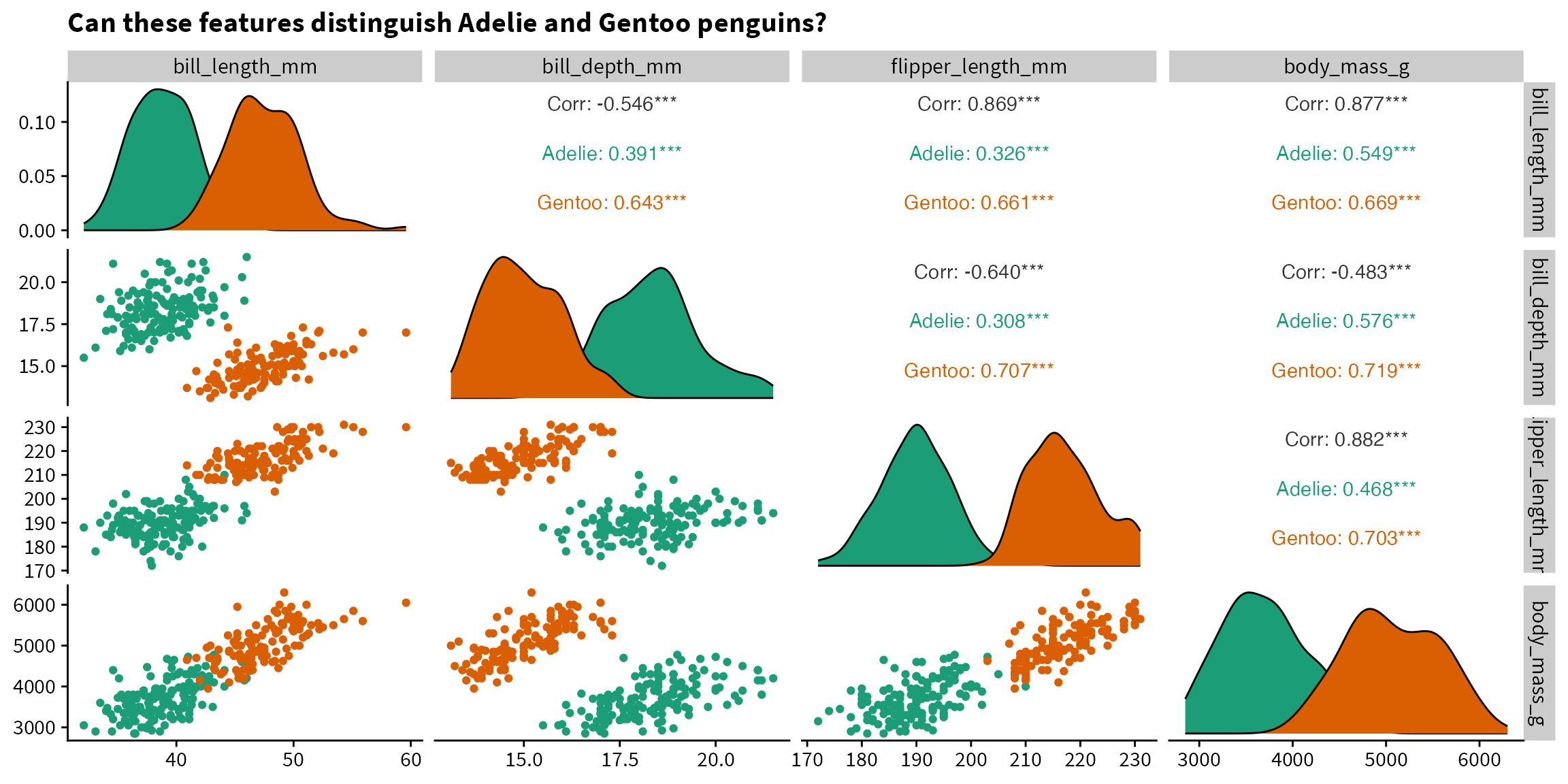

In order to help our algorithms converge, we will put our variables on a more common scale by converting bill length to cm and body mass to kg.

Code

df$bill_length_cm <- df$bill_length_mm / 10
df$body_mass_kg <- df$body_mass_g / 1000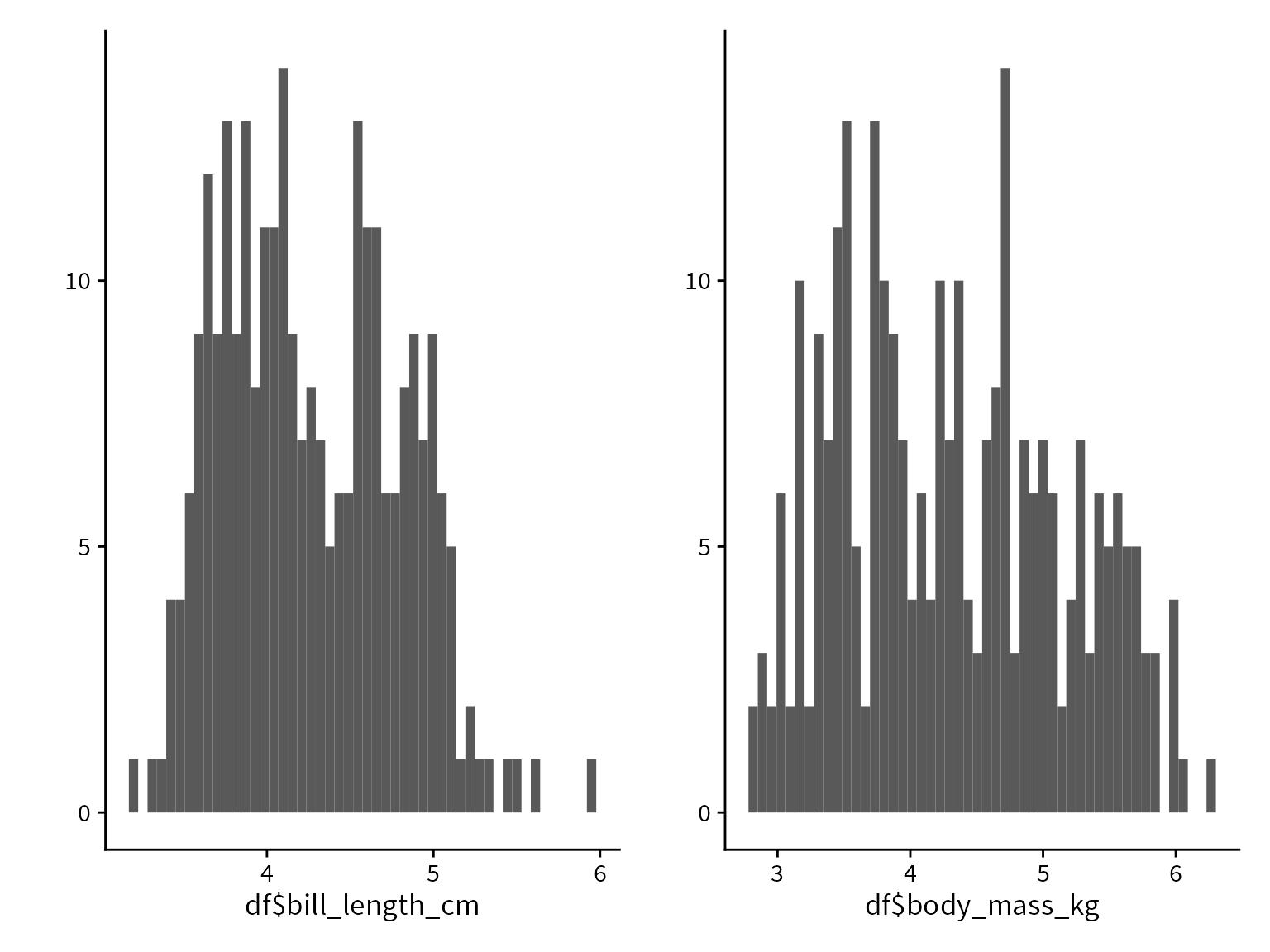

Code

# Look at distribution of bill length in cm and body mass in kg
qplot(df$bill_length_cm,bins=50) + qplot(df$body_mass_kg, bins=50)

Logistic regression overview

Logistic regression is a type of linear model². In statistics, a linear model means linear in the parameters, so we are modeling the output as a linear function of the parameters.

² Specifically, logistic regression is a type of generalized linear model (GLM) along with probit regression, Poisson regression, and other common models used in data analysis.

For example, if we were predicting bill length, we could create a linear model where bill length is normally distributed, with a mean determined as a linear function of body mass and species.

$\begin{matrix} μ_{i} = β_{0} + β_{1} [Body Mass]_{i} + β_{2} [Species = Adelie]_{i} \\ [Bill Length]_{i} \sim N (μ_{i}, σ^{2}) \end{matrix}$

We have three parameters, $β_{0}$ , $β_{1}$ , and $β_{2}$ . We can determine the likelihood of the data given these parameters. Maximizing the likelihood is the most common way to estimate the parameters from data. The idea is that we tune the parameters until we find the set of parameters that made the observed data most likely.

However, this won’t quite work if we want to predict a binary outcome like species. We could form a model like this: $\begin{matrix} p_{i} = β_{0} + β_{1} [Bill Length]_{i} + β_{2} [Body Mass]_{i} \\ [Species]_{i} \sim Bernoulli (p_{i}) \end{matrix}$ In words, each observation of a penguin is modeled as a Bernoulli random variable, where the probability of being Adelie is a linear function of bill length and body mass. The issue with this model is that if we let the parameters vary, the value of $p_{i}$ can exceed the range $[0, 1]$ , which doesn’t make sense if we are trying to model a probability.

The solution is using the expit function: $expit = \frac{e^{x}}{1 + e^{x}}$

This function takes in a real valued input and transforms it to lie within the range $[0, 1]$ . The expit function is also called the logistic function, hence the name “logistic regression”.

Let’s try it out in an example.

Code

# This is a naive implementation that can overflow for large x
# expit <- function(x) exp(x) / (1 + exp(x))

# Better to use the built-in version
expit <- plogis

Code

# Plot the output of the expit() function for x values between -10 and 10
x <- seq(-10, 10, length.out=1e5)
plot(x,
     expit(x),
     type = "l",
     main = "Understanding the effect of expit")

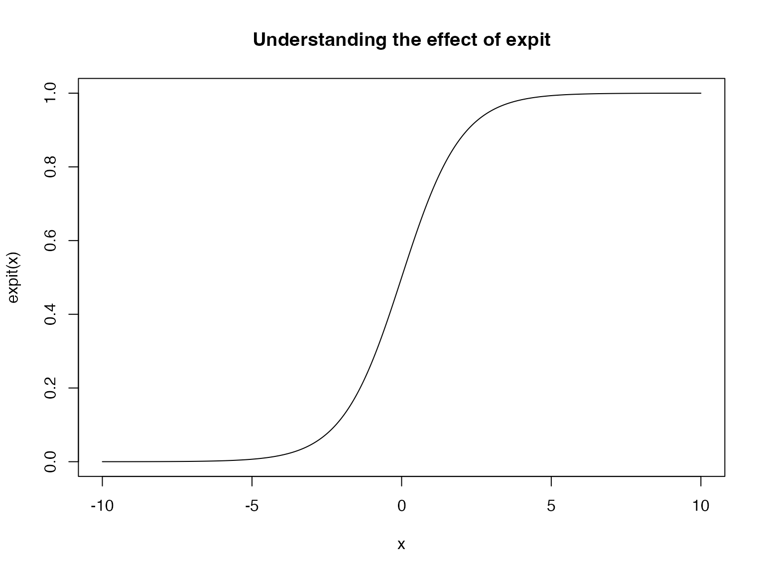
We see that (approximately) anything below -5 gets squashed to zero and anything above 5 gets squashed to 1.

We then modify our model to be $\begin{matrix} p_{i} = expit (β_{0} + β_{1} [Bill Length] + β_{2} [Body Mass]) \\ [Species] \sim Bernoulli (p_{i}) \end{matrix}$ so now $p_{i}$ is constrained to lie within $[0, 1]$ . This type of model, where we take a linear function of the parameters and then apply a non-linear function to it, is known as a generalized linear model (GLM).

The likelihood contribution of a single observation is $p_{i}$ if it is Adelie and $1 - p_{i}$ if it is Gentoo, which we can write as

${Likelihood}_{i} = p_{i}^{Adelie} (1 - p_{i})^{1 - Adelie}$

This form of writing the Bernoulli PMF works because if Adelie = 1, then ${Likelihood}_{i} = p_{i}^{1} (1 - p_{i})^{1 - 1} = p_{i}$ and if Adelie = 0, then ${Likelihood}_{i} = p_{i}^{0} (1 - p_{i})^{1 - 0} = 1 - p_{i}$ .

and therefore the log-likelihood contribution of a single observation is

${Log-Likelihood}_{i} = [{[Adelie]}_{i} \times \log (p_{i})] + [(1 - {[Adelie]}_{i}) \times \log (1 - p_{i})]$

The log-likelihood of the entire dataset is just the sum of all the individual log-likelihoods, since we are assuming independent observations, so we have

$Log-Likelihood = \sum_{i = 1}^{n} [[{[Adelie]}_{i} \times \log (p_{i})] + [(1 - {[Adelie]}_{i}) \times \log (1 - p_{i})]]$

and now substituting in $p_{i}$ in terms of the parameters, we have $\begin{aligned} Log-Likelihood & = \sum_{i = 1}^{n} [\underset{Contribution from Adelie observations}{\underset{⏟}{[{[Adelie]}_{i} \times \log (expit (β_{0} + β_{1} [Bill Length]_{i} + β_{2} [Body Mass]_{i}))]}} \\ + \underset{Contribution from Gentoo observations}{\underset{⏟}{[(1 - {[Adelie]}_{i}) \times \log (1 - expit (β_{0} + β_{1} [Bill Length]_{i} + β_{2} [Body Mass]_{i}))]}}] \end{aligned}$

We can then pick $β_{0}$ , $β_{1}$ , and $β_{2}$ to maximize this log-likelihood function, or as is often done in practice, minimize the negative log-likelihood function. We will need to do this with numerical methods, rather than obtaining an analytical solution with calculus, since no closed-form solution exists.

Logistic regression with `glm()`

Before we implement logistic regression by hand, we will use the glm() function in R as a baseline. Under the hood, R uses the Fisher Scoring Algorithm to obtain the maximum likelihood estimates.

Code

# Fit the logistic regression model
model_glm <- glm(adelie ~ bill_length_cm + body_mass_kg,
                 family=binomial(link = "logit"),
                 data=df)

Now that we have fit the model, let’s look at the predictions of the model. We can make a grid of covariate values, and ask the model to give us the predicted probability of Species = Adelie for each one.

Code

# Create a grid of values on which to evaluate probabilities
grid <-
crossing(bill_length_cm = seq(min(df$bill_length_cm)-0.2, max(df$bill_length_cm)+0.2, 0.001),
         body_mass_kg = seq(min(df$body_mass_kg)-0.1, max(df$body_mass_kg)+0.1, 0.005))

We use the predict() function to obtain the predicted probabilities. Using type = "response" specifies that we want the predictions on the probability scale (i.e., after passing the linear predictor through the expit function.).

Code

grid$predicted <- predict(model_glm, grid, type = "response")

bill_length_cm	body_mass_kg	predicted
5.287	6.105	0.0000001
5.755	2.840	0.0022277
5.657	5.825	0.0000000
4.462	4.905	0.0298950
4.519	6.065	0.0001169
6.130	3.090	0.0000257
6.092	4.370	0.0000001
5.616	6.050	0.0000000
5.533	4.675	0.0000055
3.442	5.815	0.8491884
4.557	3.765	0.6546862
4.358	3.360	0.9851913
3.477	6.020	0.6268662
5.550	3.805	0.0002095
4.230	3.785	0.9705454
5.127	6.315	0.0000002
5.961	3.870	0.0000039
5.010	4.880	0.0002480
5.167	4.430	0.0004301
4.263	4.605	0.4061394
4.620	2.835	0.9841835
5.678	4.025	0.0000254
5.131	5.045	0.0000406
4.408	3.405	0.9721137
5.389	3.790	0.0009517
5.665	3.765	0.0000886
5.761	5.505	0.0000000
3.427	5.460	0.9680849
5.227	4.880	0.0000352
4.676	4.290	0.0616915
3.896	5.735	0.1183568
5.180	4.980	0.0000347
5.415	5.100	0.0000025
6.023	3.875	0.0000022
5.420	6.360	0.0000000
4.552	4.990	0.0093732
6.091	4.235	0.0000002
3.870	4.635	0.9537189
3.853	6.050	0.0476244
4.815	6.290	0.0000031
3.967	5.675	0.0843093
3.115	5.355	0.9987433
3.299	4.345	0.9999197
4.809	3.710	0.1997304
4.837	4.660	0.0030633
5.581	5.730	0.0000000
3.797	4.505	0.9859334
4.694	2.875	0.9640952
3.320	4.840	0.9991593
4.583	2.790	0.9906229
4.185	5.960	0.0037194
3.292	5.390	0.9928432
3.282	3.575	0.9999976
4.709	3.975	0.1618652
4.154	5.960	0.0049102
4.552	2.830	0.9915448
4.398	5.740	0.0014320
3.052	6.130	0.9794326
6.015	3.260	0.0000344
4.159	5.855	0.0074037
4.354	3.515	0.9722746
5.859	4.545	0.0000005
4.807	3.205	0.6971030
5.838	5.110	0.0000001
4.537	3.715	0.7384344
4.324	3.945	0.8755539
3.760	4.185	0.9974751
4.820	3.090	0.7717730
4.623	5.070	0.0035106
4.036	6.190	0.0052033
6.145	4.945	0.0000000
4.555	4.835	0.0177903
6.054	3.085	0.0000520
4.706	3.920	0.2014218
5.669	2.995	0.0024554
4.568	4.730	0.0248441
5.785	3.630	0.0000543
3.620	3.245	0.9999881
5.188	4.825	0.0000635
5.144	6.030	0.0000005
4.999	3.615	0.0639715
6.022	6.100	0.0000000
4.351	3.780	0.9189363
6.035	4.170	0.0000005
4.533	4.725	0.0344495
5.689	4.160	0.0000127
5.407	5.570	0.0000003
3.911	4.500	0.9625201
3.749	4.335	0.9956077
5.552	5.745	0.0000000
5.122	6.180	0.0000003
3.918	4.625	0.9332259
5.408	2.965	0.0285411
4.192	4.515	0.6573858
4.271	4.180	0.8025823
5.068	5.340	0.0000198
5.500	3.905	0.0002124
4.897	5.295	0.0001121
4.881	5.770	0.0000163
3.734	6.205	0.0690677
3.611	3.320	0.9999848
4.886	6.345	0.0000013
4.080	3.250	0.9992383
4.767	4.825	0.0028003
4.130	2.910	0.9997289
5.421	4.875	0.0000063
3.676	3.510	0.9999375
5.557	3.725	0.0002789
5.320	4.835	0.0000185
6.129	5.795	0.0000000
3.630	3.565	0.9999475
4.129	3.040	0.9995264
4.154	5.745	0.0124515
4.196	3.350	0.9966620
5.988	2.820	0.0002992
5.690	5.445	0.0000000
5.984	6.300	0.0000000
3.060	3.565	0.9999997
4.456	6.390	0.0000499
5.438	6.260	0.0000000
4.113	4.120	0.9563162
5.717	5.045	0.0000002
3.565	5.730	0.7295421
4.147	5.665	0.0186824
5.093	4.645	0.0003276
4.597	4.685	0.0233260
3.761	4.955	0.9315152
5.658	6.305	0.0000000
4.344	4.125	0.7282171
5.474	3.295	0.0038291
4.507	2.870	0.9932731
5.661	5.665	0.0000000
5.026	3.465	0.0934974
3.544	3.975	0.9998551
3.012	4.840	0.9999474
4.975	6.395	0.0000005
4.090	5.605	0.0396736
5.575	3.145	0.0029717
5.280	2.835	0.1408342
3.980	5.415	0.2029946
4.258	5.770	0.0044150
3.699	4.095	0.9990138
4.102	5.925	0.0090953
3.902	3.265	0.9998360
5.447	6.125	0.0000000
3.768	4.290	0.9957173
5.557	3.495	0.0007604
3.714	5.900	0.2515647
3.159	5.185	0.9991104
3.248	5.330	0.9962798
3.642	5.820	0.4766904
6.032	5.700	0.0000000
5.133	4.245	0.0013080
4.436	3.130	0.9890056
3.985	4.550	0.9138578
3.517	2.930	0.9999988
3.224	5.535	0.9926940
4.313	6.095	0.0006542
3.398	3.685	0.9999890
5.902	4.725	0.0000002
3.988	5.290	0.2902346
4.044	2.950	0.9998511
4.945	4.070	0.0150290
5.294	5.270	0.0000035
5.089	3.955	0.0068499
5.898	3.965	0.0000046
5.198	5.745	0.0000010
4.600	3.155	0.9485557
4.088	4.580	0.7864920
6.091	5.140	0.0000000
4.000	2.960	0.9998953
5.637	4.175	0.0000191
4.899	4.180	0.0140821
4.033	4.820	0.6795311
4.439	4.805	0.0553886
5.062	6.345	0.0000003
4.060	5.130	0.3006920
3.703	3.485	0.9999285
4.389	5.585	0.0030489
4.853	3.350	0.4469271
5.445	2.915	0.0255251
3.892	3.755	0.9987300
4.750	4.125	0.0648959
5.812	3.925	0.0000117
5.153	5.090	0.0000274
5.506	6.315	0.0000000
5.427	3.025	0.0187022
4.570	4.230	0.1814927
4.618	3.130	0.9459126
3.347	5.420	0.9867009
3.997	5.325	0.2445391
5.281	3.210	0.0306600
4.710	2.955	0.9425279
3.492	5.755	0.8234821
5.227	6.175	0.0000001
4.670	4.955	0.0037975
5.405	3.075	0.0183351
3.841	4.875	0.9037304
5.406	4.850	0.0000080
4.031	5.600	0.0669916

Now that we have the predictions, let’s plot them and overlay the data with their true labels. The model looks to be performing pretty well!

Code

grid %>%
  ggplot() +
  aes(x=bill_length_cm,
      y=body_mass_kg) +
  geom_raster(aes(fill=predicted)) +
  geom_point(data=df, mapping = aes(color=species)) +
  geom_point(data=df, color="black", shape=21) +
  scale_fill_viridis_c(breaks = seq(0, 1, 0.25),
                       limits=c(0,1)) +
  scale_color_brewer(palette="Dark2") +
  scale_x_continuous(breaks=seq(3, 6, 0.5)) +
  scale_y_continuous(breaks=seq(3, 6, 0.5)) +
  labs(fill = "Probability of Adelie\n",
       color = "Species",
       x = "Bill length (mm)",
       y = "Body mass (g)",
       title = "Visualizing the predictions of the logistic regression model") +
  theme(legend.key.height = unit(1, "cm"))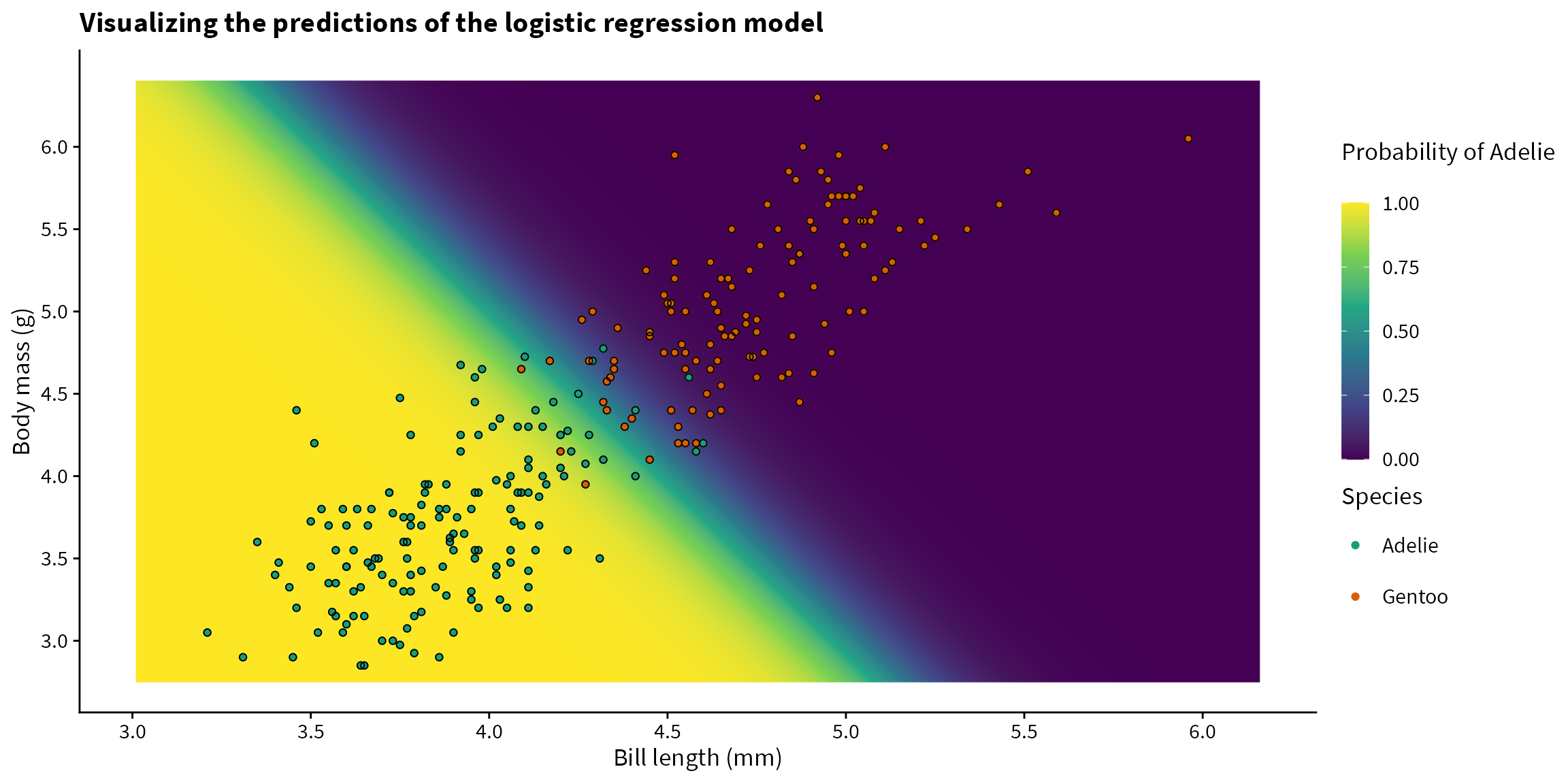

Logistic regression with `optim()`

Now that we know what to expect after using glm(), let’s implement logistic regression by hand.

Recall that we would like to numerically determine the beta values that minimize the negative log-likelihood. The optim() function in R is a general-purpose function for minimizing functions³.

³ This short video is a good introduction to optim().

⁴ Sourced from here

optim() has an algorithm called Nelder-Mead that searches the parameter space and converges on the minimum value. It is a direct search method that only requires the negative log-likelihood function as input (as opposed to gradient based methods that require specified the gradients of the negative log-likelihood function). This animation demonstrates the Nelder-Mead algorithm in action⁴.

Nelder-Mead animation

To use optim(), we create a function that takes as input the parameters and returns the negative log-likelihood. The below code is a translation of the mathematical notation from above.

Code

neg_loglikelihood_function <- function(parameters){
  
  # optim() expects the parameters as a single vector, so we set the coefficients
  # as the elements of a vector called `parameters`
  b0 <- parameters[1]
  b1 <- parameters[2]
  b2 <- parameters[3]
  
  linear_predictor <- (b0) + (b1*df$bill_length_cm) + (b2*df$body_mass_kg)
  
  # Likelihood for each observation
  # If the observation is Adelie, then the likelihood is the probability of Adelie
  # If the observation is not Adelie (i.e., Gentoo), then the likelihood is the probability of not Adelie
  # which is 1 - P(Adelie)
  likelihood <- ifelse(df$adelie==1,
                       expit(linear_predictor),
                       1-expit(linear_predictor))
  
  # Log-likelihood for each observation
  log_likelihood <- log(likelihood)
  
  # Joint log-likelihood for all the observations. Note the sum because
  # multiplication is addition on the log-scale
  total_log_likelihood <- sum(log_likelihood)
  
  # the optim() function only minimizes, so we return the negative log-likelihood
  # and then maximize it
  return(-total_log_likelihood)
}

As an example, we can pass in $β_{0} = 1, β_{1} = 2, β_{2} = 3$ and see what the negative log-likelihood is.

Code

neg_loglikelihood_function(c(1,2,3))

[1] 3164.666

Because the negative log-likelihood is very high, we know that these are poor choices for the parameter values.

We can visualize the negative log-likelihood function for a variety of values. Since there are 3 parameters in our model, and we cannot visualize in 4D, we set $β_{0} = 58.075$ , which was the optimized value found by glm() and we can visualize how the negative log-likelihood varies with $β_{1}$ and $β_{2}$ .

Code

# Create a grid of parameter values
grid <-
  crossing(
    b0 = 58.075,
    b1 = seq(-12, -7, length.out=1e2),
    b2 = seq(-6, -2, length.out=1e2)
  )

Code

# Evaluate the negative log-likelihood for each parameter value
grid$neg_loglikelihood <-
  pmap_dbl(grid,
           ~neg_loglikelihood_function(c(..1, ..2, ..3)))

Code

# Show a heatmap of the negative log-likelihood with contour lines
grid %>%
  ggplot() +
  aes(x=b1,
      y=b2) +
  geom_raster(aes(fill=neg_loglikelihood)) +
  geom_contour(aes(z=neg_loglikelihood), bins = 50, size=0.1, color="gray") +
  scale_fill_viridis_c() +
  scale_color_brewer(palette="Dark2") +
  annotate(geom="point", x=-8.999, y=-4.363, color="red") +
  labs(fill = "Negative log-likelihood\n",
       x = "Beta 1",
       y = "Beta 2",
       title = "Visualizing the negative log-likelihood function") +
  theme(legend.key.height = unit(1, "cm"))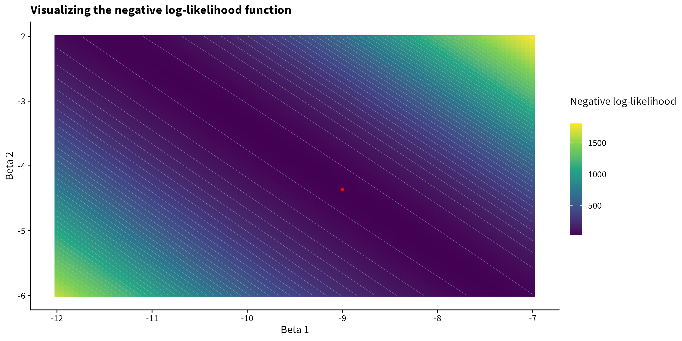

To use optim(), we pass in the starting parameter values to par and the function to be minimized (the negative log-likelihood) to fn. Finally, we’ll specify method="Nelder-Mead".

Code

optim_results <-
  optim(par=c(0,0,0),                      # Initial values
        fn = neg_loglikelihood_function,   # Objective function to be minimized
        method="Nelder-Mead")              # Optimization method

The maximum likelihood estimates are stored in the $par attribute of the optim object

Code

optim_results$par

[1] 58.080999 -9.001399 -4.362164

which we can compare with the coefficients obtained from glm(), and we see that they match quite closely.

Code

coef(model_glm)

   (Intercept) bill_length_cm   body_mass_kg 
     58.074991      -8.998692      -4.363412

The below animation demonstrates the path of the Nelder-Mead function⁵. As stated above, for the purpose of the animation, we set the optimized value of $β_{0} = 58.075$ and we can visualize how the negative log-likelihood is optimized with respect to $β_{1}$ and $β_{2}$ .

⁵ The code for this animation is long, so it is not included here, but can be viewed in the source code of the Quarto document.

Animation of the path taken by the Nelder Mead algorithm

Logistic regression with gradient descent

Going one step further, instead of using a built-in optimization algorithm, let’s maximize the likelihood ourselves using gradient descent. If you need a refresher, I have written a blog post on gradient descent which you can find here.

We need the gradient of the negative-log likelihood function. The slope with respect to the jth parameter is given by

$\begin{array}{r} [expit (β \cdot x) - y] x_{j} ⟹ [\hat{y} - y] x_{j} \end{array}$ so then the gradient can be written as $\begin{array}{r} X^{T} [expit (X β) - y] \end{array}$ or equivalently $\begin{array}{r} X^{T} (\hat{y} - y) \end{array}$

You can find a nice derivation of the derivative of the negative log-likelihood for logistic regression here.

Another approach is to use automatic differentiation. Automatic differentiation can be used to obtain gradients for arbitrary functions, and is used heavily in deep learning. An example to do this in R using the torch library is shown here.

We implement the above equations in the following function for the gradient.

Code

gradient <- function(parameters){
  # Given a vector of parameters values, return the current gradient
  
  b0 <- parameters[1]
  b1 <- parameters[2]
  b2 <- parameters[3]
  
  # Define design matrix
  X <- cbind(rep(1, nrow(df)),
                 df$bill_length_cm,
                 df$body_mass_kg)
  
  beta <- matrix(parameters)
  
  y_hat <- expit(X %*% beta)
  
  gradient <- t(X) %*% (y_hat - df$adelie)
  
  return(gradient)
}

We must specify type="2" in the norm() function to specify that we want the Euclidean length of the vector.

Now we implement the gradient descent algorithm. We stop if the difference between the new parameter vector and old parameter vector is less than $10^{- 6}$ .

Code

set.seed(777)

step_size <- 0.001   # Learning rate
theta <- c(0,0,0)    # Initial parameter value
iter <- 1

while (TRUE) {
  iter <- iter + 1
  current_gradient <- gradient(theta)               
  
  theta_new <- theta - (step_size * current_gradient)
  
  if (norm(theta - theta_new, type="2") < 1e-6) {
    break
  } else{
    theta <- theta_new
  }
}

Code

print(glue("Number of iterations: {iter}"))

Number of iterations: 541366

Code

print(glue("Final parameter values: {as.numeric(theta)}"))

Final parameter values: 57.9692967372787
Final parameter values: -8.98174736147028
Final parameter values: -4.35607256440227

Code

print(glue("`glm()` parameter values (for comparison): {as.numeric(coef(model_glm))}"))

`glm()` parameter values (for comparison): 58.0749906489601
`glm()` parameter values (for comparison): -8.99869242178258
`glm()` parameter values (for comparison): -4.36341215126915

Again, we see that the results are very close to the glm() results.

Conclusion

Hopefully this post was helpful for understanding the inner workings of logistic regression and how the principles can be extended to other types of models. For example, Poisson regression is another type of generalized linear model just like logistic regression, where in that case we use the exp function instead of the expit function to constrain parameter values to lie in the range $[0, \infty]$ .

Overview

Data

Exploratory data analysis

Logistic regression overview

Logistic regression with glm()

Logistic regression with optim()

Logistic regression with gradient descent

Conclusion

Logistic regression with `glm()`

Logistic regression with `optim()`